分析光波由光疏介质进入光密介质时反射率和透射率的变化。光疏介质空气 $n_1=1$,光密介质石英玻璃 $n_2=1.45$,作出 $p$、$s$ 分量的振幅反射率和振幅透射率以及他们的绝对值随入射角度的变化曲线。
 1
 2
 3
 4
 5
 6
 7
 8
 9
10
11
12
13
14
15
16
17
18
19
20
21
22
23
24
| n1=1, n2=1.45;
theta=0:0.1:90;
a=theta*pi/180;
rp=(n2*cos(a)-n1*sqrt(1-(n1/n2*sin(a)).^2))./(n2*cos(a)+n1*sqrt(1-(n1/n2*sin(a)).^2));
rs=(n1*cos(a)-n2*sqrt(1-(n1/n2*sin(a)).^2))./(n1*cos(a)+n2*sqrt(1-(n1/n2*sin(a)).^2));
tp=2*n1*cos(a)./(n2*cos(a)+n1*sqrt(1-(n1/n2*sin(a)).^2));
ts=2*n1*cos(a)./(n1*cos(a)+n2*sqrt(1-(n1/n2*sin(a)).^2));
figure(1);
subplot(1,2,1);
plot(theta,rp,'-',theta,rs,'--',theta,abs(rp),':',theta,abs(rs),'-.','LineWidth',2)
legend('r_p','r_s','|r_p|','|r_s|')
xlabel('\theta_i')
ylabel('Amplitude')
title(['n_1=',num2str(n1),',n_2=',num2str(n2)])
axis([0 90 -1 1])
grid on
subplot(1,2,2);
plot(theta,tp,'-',theta,ts,'--',theta,abs(tp),':',theta,abs(ts),'-.','LineWidth',2)
legend('t_p','t_s','|t_p|','|t_s|')
xlabel('\theta_i')
ylabel('Amplitude')
title(['n_1=',num2str(n1),',n_2=',num2str(n2)])
axis([0 90 0 1])
grid on
|
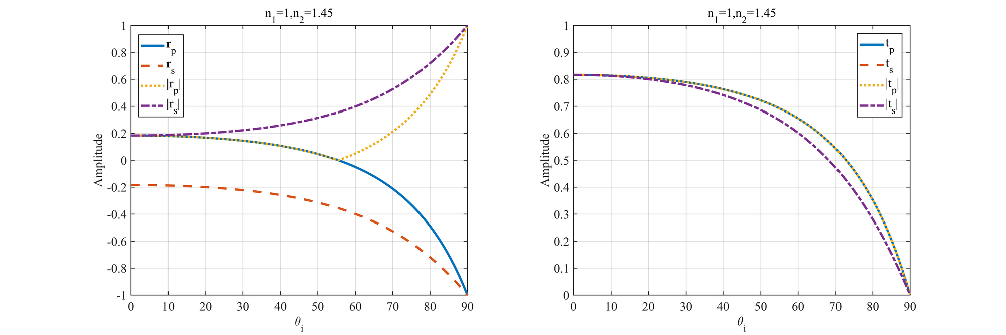
由图可知:
- 当入射角 $\theta_i=0$,即垂直入射时,$r_p$、$r_s$ 和 $t_p$、$t_s$ 都不为 $0$,表示存在反射波和折射波。
- 当入射角 $\theta_i=90$,即掠入射时,$r_p=r_s=-1$,$t_p=t_s=0$,即没有折射光波。
- $t_p$、$t_s$ 随 $\theta_i$ 的增大而减小,$|r_s|$ 随 $\theta_i$ 的增大而增大,直到等于 $1$。
- $|r_p|$ 先随 $\theta_i$ 的增大而减小,到达一特定的值 $\theta_B$ 时,有 $|r_p|=0$,即反射波中此时没有 $p$ 分量,只有 $s$ 分量,产生全偏振现象,然后随着 $\theta_i$ 的增大,$|r_p|$ 不断增大,直到等于 $1$。
作出 $p$、$s$ 分量的能流反射率和能流透射率以及他们的平均值随入射角度的变化曲线。
 1
 2
 3
 4
 5
 6
 7
 8
 9
10
11
12
13
14
15
16
17
18
19
20
21
22
23
24
25
26
27
28
29
30
| n1=1, n2=1.45;
theta=0:0.1:90;
a=theta*pi/180;
rp=(n2*cos(a)-n1*sqrt(1-(n1/n2*sin(a)).^2))./(n2*cos(a)+n1*sqrt(1-(n1/n2*sin(a)).^2));
rs=(n1*cos(a)-n2*sqrt(1-(n1/n2*sin(a)).^2))./(n1*cos(a)+n2*sqrt(1-(n1/n2*sin(a)).^2));
tp=2*n1*cos(a)./(n2*cos(a)+n1*sqrt(1-(n1/n2*sin(a)).^2));
ts=2*n1*cos(a)./(n1*cos(a)+n2*sqrt(1-(n1/n2*sin(a)).^2));
Rp=abs(rp).^2;
Rs=abs(rs).^2;
Rn=(Rp+Rs)/2;
Tp=n2*sqrt(1-(n1/n2*sin(a)).^2)./(n1*cos(a)).*abs(tp).^2;
Ts=n2*sqrt(1-(n1/n2*sin(a)).^2)./(n1*cos(a)).*abs(ts).^2;
Tn=(Tp+Ts)/2;
figure(1);
subplot(1,2,1);
plot(theta,Rp,'-',theta,Rs,'-.',theta,Rn,'--','LineWidth',2)
legend('R_p','R_s','R_n')
xlabel('\theta_i')
ylabel('Amplitude')
title(['n_1=',num2str(n1),',n_2=',num2str(n2)])
axis([0 90 0 1])
grid on
subplot(1,2,2);
plot(theta,Tp,'-',theta,Ts,'-.',theta,Tn,'--','LineWidth',2)
legend('T_p','T_s','T_n')
xlabel('\theta_i')
ylabel('Amplitude')
title(['n_1=',num2str(n1),',n_2=',num2str(n2)])
axis([0 90 0 1])
grid on
|
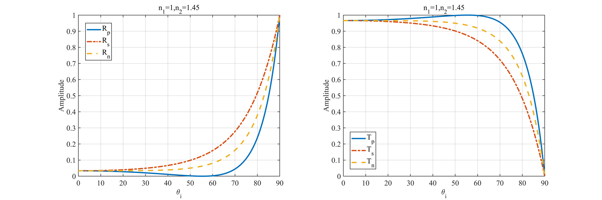
由图可知:
- 当入射角 $\theta_i=0$ 时,垂直入射时能流反射率 $R_p$、$R_s$ 和 $T_p$、$T_s$ 都不为 $0$,此时存在反射光波。
- 随着 $\theta_i$ 的增大,$R_s$ 不断增大至 $1$,$T_s$ 不断减小至 $0$,但始终有 $R_s+T_s=1$。
- 随着 $\theta_i$ 的增大,$R_p$ 先减小,直至一特定的值 $\theta_B$ 时变为 $0$,而后随着 $\theta_i$ 的增大不断增大到 $1$。$T_p$ 的过程正好相反,在入射角为 $\theta_B$ 时为 $1$,且始终有 $R_p+T_p=1$。
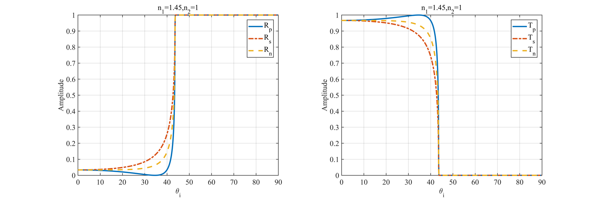
分析光波由光密介质进入光疏介质时反射率和透射率的变化。光疏介质空气 $n_1=1$,光密介质石英玻璃 $n_2=1.45$,作出 $p$、$s$ 分量的振幅反射率和振幅透射率以及他们的绝对值随入射角度的变化曲线。
与上述过程相同,只需要将折射率互换。此处的光波变化分析略去。
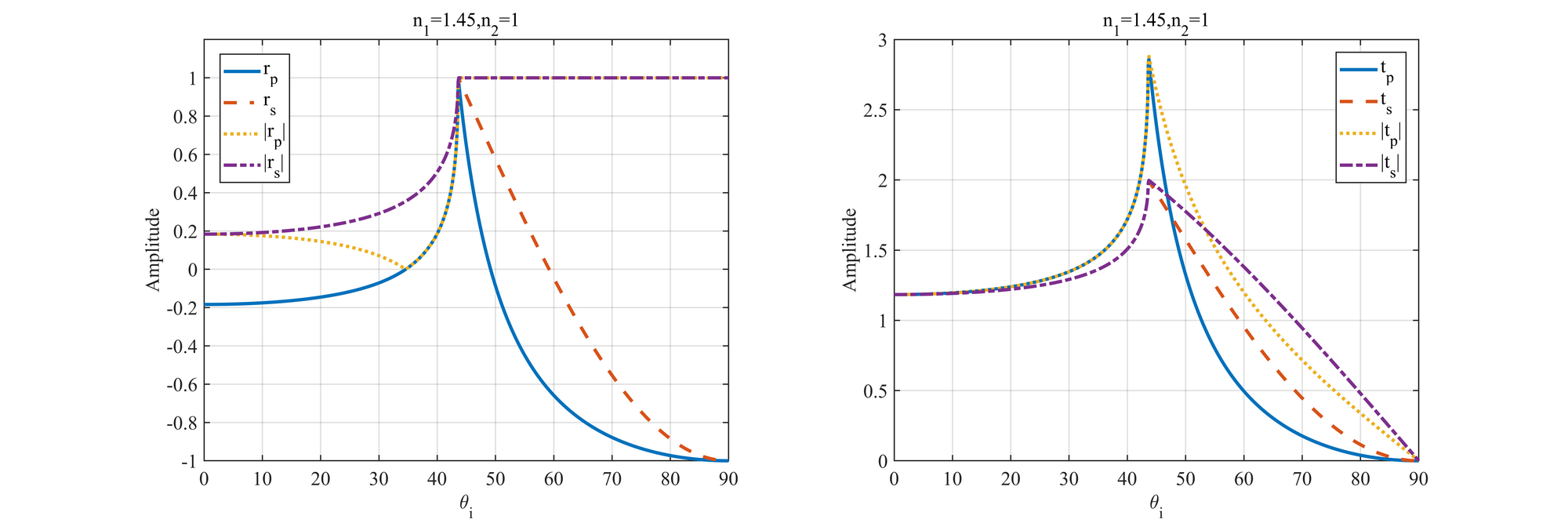
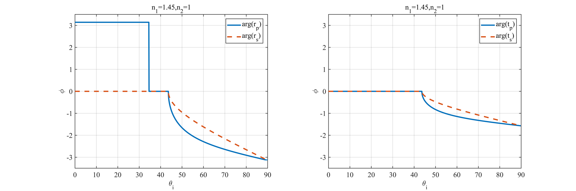
在图中,$\theta_i>\theta_c$ 后,$|r_p|$ 和 $r_p$ 以及 $|r_s|$ 和 $r_s$ 产生了很大的差异。因为 $n_1>n_2$, 如果 $\sin\theta_i>n_2/n_1$ 则 $1-(n_1/n_2)^2\sin^2\theta_1<0$,计算得到的 $r_p$ 和 $r_s$ 将变为复数。但作图时只取了实部。
 1
 2
 3
 4
 5
 6
 7
 8
 9
10
11
12
13
14
15
16
17
18
19
20
21
22
23
24
25
26
27
28
29
| [theta' rp' rs']
ans =
0.0000 + 0.0000i -0.1837 + 0.0000i 0.1837 + 0.0000i
0.1000 + 0.0000i -0.1837 + 0.0000i 0.1837 + 0.0000i
0.2000 + 0.0000i -0.1837 + 0.0000i 0.1837 + 0.0000i
0.3000 + 0.0000i -0.1837 + 0.0000i 0.1837 + 0.0000i
0.4000 + 0.0000i -0.1837 + 0.0000i 0.1837 + 0.0000i
0.5000 + 0.0000i -0.1837 + 0.0000i 0.1837 + 0.0000i
......
43.0000 + 0.0000i 0.5449 + 0.0000i 0.7542 + 0.0000i
43.1000 + 0.0000i 0.5754 + 0.0000i 0.7727 + 0.0000i
43.2000 + 0.0000i 0.6108 + 0.0000i 0.7938 + 0.0000i
43.3000 + 0.0000i 0.6531 + 0.0000i 0.8185 + 0.0000i
43.4000 + 0.0000i 0.7064 + 0.0000i 0.8487 + 0.0000i
43.5000 + 0.0000i 0.7814 + 0.0000i 0.8897 + 0.0000i
43.6000 + 0.0000i 0.9601 + 0.0000i 0.9808 + 0.0000i
43.7000 + 0.0000i 0.9717 + 0.2360i 0.9935 + 0.1135i
43.8000 + 0.0000i 0.9433 + 0.3319i 0.9869 + 0.1614i
43.9000 + 0.0000i 0.9155 + 0.4023i 0.9802 + 0.1978i
44.0000 + 0.0000i 0.8883 + 0.4593i 0.9736 + 0.2283i
......
89.5000 + 0.0000i -0.9999 + 0.0115i -0.9997 + 0.0241i
89.6000 + 0.0000i -1.0000 + 0.0092i -0.9998 + 0.0193i
89.7000 + 0.0000i -1.0000 + 0.0069i -0.9999 + 0.0145i
89.8000 + 0.0000i -1.0000 + 0.0046i -1.0000 + 0.0096i
89.9000 + 0.0000i -1.0000 + 0.0023i -1.0000 + 0.0048i
90.0000 + 0.0000i -1.0000 + 0.0000i -1.0000 + 0.0000i
|
光波从光密介质入射光疏介质在一定角度会发生全反射现象,将上述程序代码中的折射率互换即可得到下图。
平面光波从石英玻璃入射到空气,空气 $n_1=1$,石英玻璃 $n_2=1.45$,作出 $p$、$s$ 分量的反射波相位和透射波相位随入射角度的变化曲线。
 1
 2
 3
 4
 5
 6
 7
 8
 9
10
11
12
13
14
15
16
17
18
19
20
21
22
23
24
25
26
27
28
| n1=1, n2=1.45;
theta=0:0.1:90;
a=theta*pi/180;
rp=(n2*cos(a)-n1*sqrt(1-(n1/n2*sin(a)).^2))./(n2*cos(a)+n1*sqrt(1-(n1/n2*sin(a)).^2));
rs=(n1*cos(a)-n2*sqrt(1-(n1/n2*sin(a)).^2))./(n1*cos(a)+n2*sqrt(1-(n1/n2*sin(a)).^2));
tp=2*n1*cos(a)./(n2*cos(a)+n1*sqrt(1-(n1/n2*sin(a)).^2));
ts=2*n1*cos(a)./(n1*cos(a)+n2*sqrt(1-(n1/n2*sin(a)).^2));
arp=angle(rp);
ars=angle(rs);
atp=angle(tp);
ats=angle(ts);
figure(1);
subplot(1,2,1);
plot(theta,arp,'-',theta,ars,'--','LineWidth',2)
legend('arg(r_p)','arg(r_s)')
xlabel('\theta_i')
ylabel('\phi')
title(['n_1=',num2str(n1),',n_2=',num2str(n2)])
axis([0 90 -3.5 3.5])
grid on
subplot(1,2,2);
plot(theta,atp,'-',theta,ats,'--','LineWidth',2)
legend('arg(t_p)','arg(t_s)')
xlabel('\theta_i')
ylabel('\phi')
title(['n_1=',num2str(n1),',n_2=',num2str(n2)])
axis([0 90 -3.5 3.5])
grid on
|
作出束腰半径为 $0.5mm$ 的高斯光束在束腰处的三维光强分布图。
 1
 2
 3
 4
 5
 6
 7
 8
 9
10
11
12
13
14
15
| N=200;
w0=0.5;
r=linspace(0,3*w0,N);
eta=linspace(0,2*pi,200);
[rho,theta]=meshgrid(r,eta);
[x,y]=pol2cart(theta,rho);
I=exp(-2*rho.^2/w0^2);
surf(x,y,I)
shading interp
xlabel('position /mm')
ylabel('position /mm')
zlabel('relative intensity /a.u.')
title('Causs intensity distribution')
axis([-3*w0 3*w0 -3*w0 3*w0 0 1])
colorbar
|
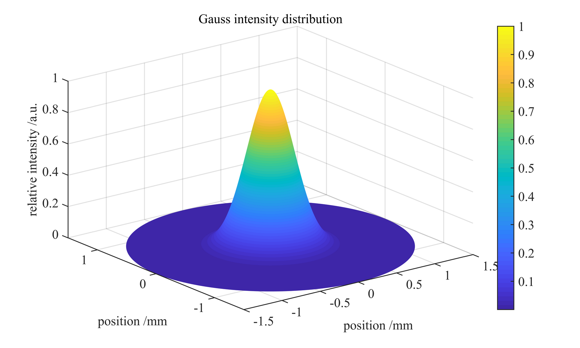 ※ 高斯光束的三维光强分布
作出束腰半径为 $0.5mm$ 的高斯光束在束腰处的二维光强分布图。
 1
 2
 3
 4
 5
 6
 7
 8
 9
10
11
12
13
14
15
16
| Npoint=501;
w0=0.5;
x=linspace(-3*w0,3*w0,Npoint);
y=linspace(-3*w0,3*w0,Npoint);
X=meshgrid(x,y);
Y=meshgrid(y,x);
Y=Y';
R=sqrt(X.^2+Y.^2);
I=exp(-2*R.^2/w0^2);
imagesc(x,y,I,[0 1]);
colormap gray;
colorbar
xlabel('x /mm')
ylabel('y /mm')
title('Gauss intensity distribution')
axis([-3*w0 3*w0 -3*w0 3*w0])
|
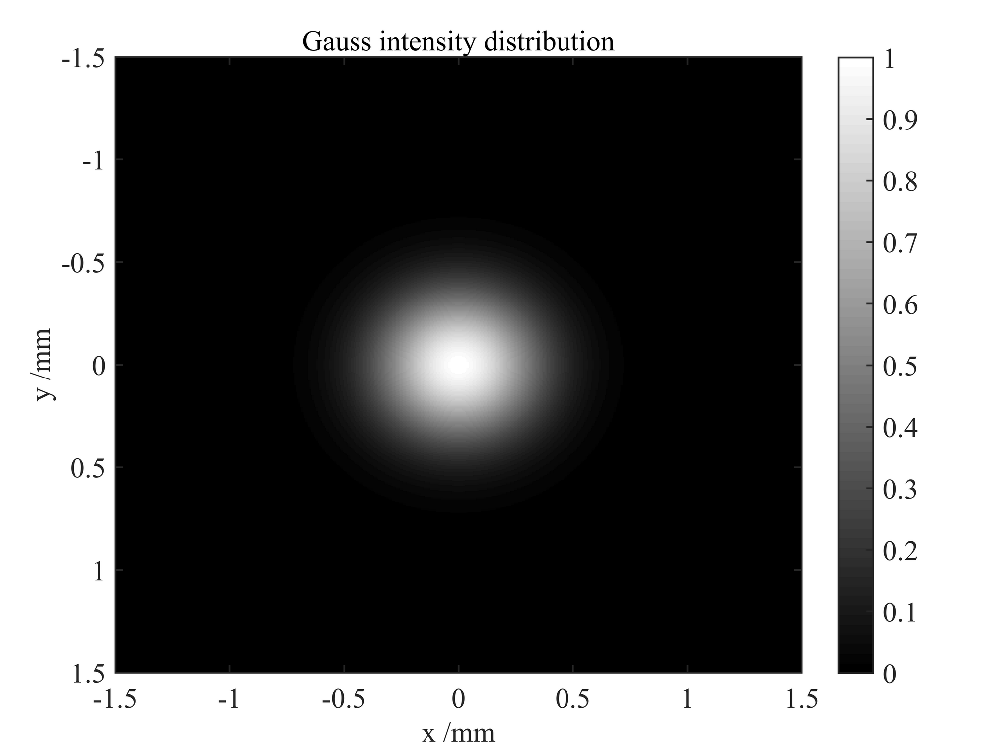 ※ 高斯光束的二维光强分布
作出束腰为 $0.5mm$,波长为 $1.55\mu m$ 的高斯光束在 $3$ 倍瑞利长度范围内传播过程中的振幅变化图。
 1
 2
 3
 4
 5
 6
 7
 8
 9
10
11
12
13
14
15
16
| w0=0.5e-3;
lambda=1.55e-6;
ZR=pi*w0^2/lambda;
Lz=3*ZR;
N=200;
z=linspace(-Lz,Lz,N);
y=linspace(-4*w0,4*w0,N);
[py,pz]=meshgrid(y,z);
wz=w0*sqrt(1+(lambda*pz/pi/w0^2).^2);
Iopt=w0^2./wz.^2.*exp(-2*py.^2./wz.^2);
imagesc(z,y,Iopt');
xlabel('z /mm');
ylabel('y /mm');
title('Intensity of Gauss beam propagation');
colorbar
colormap hot;
|
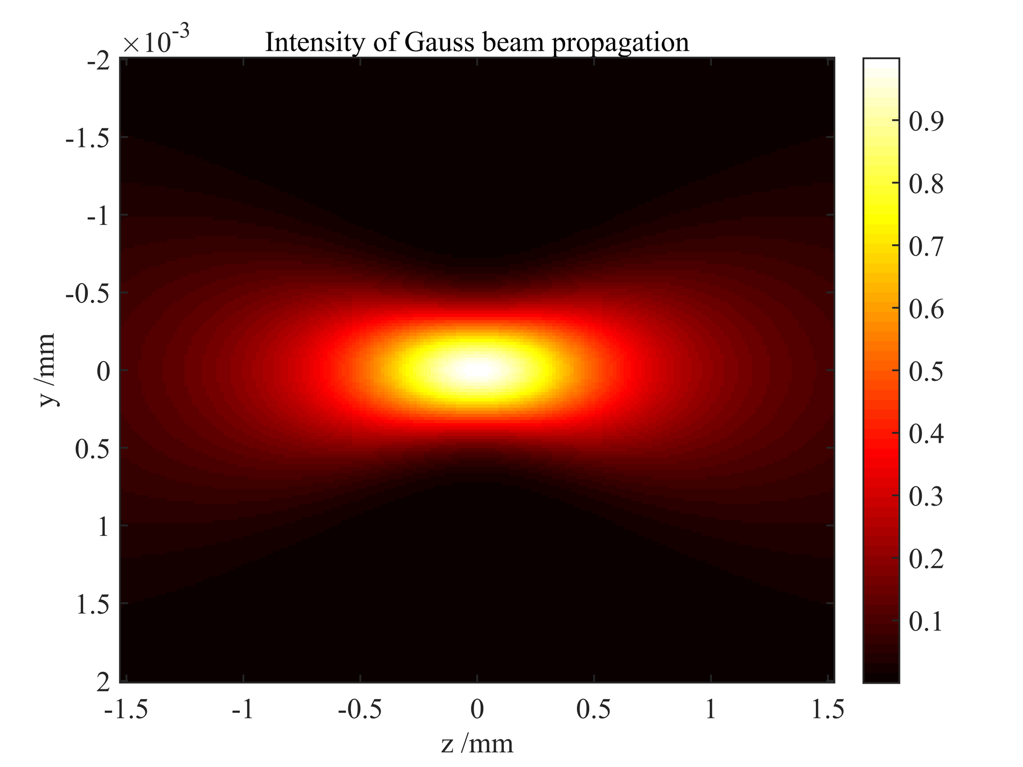 ※ 高斯光束在自由空间传播过程的光强分布
作出束腰半径为 $2\mu m$,波长为 $1.5\mu m$ 的高斯光束在自由空间传播过程中其束腰附近某一时刻的电场分量的归一化空间分布。
 1
 2
 3
 4
 5
 6
 7
 8
 9
10
11
12
13
14
15
16
17
18
19
20
21
22
23
24
| lambda=1.5e-6;
w0=2e-6;
Ld=10*w0;
Rd=5*w0;
N=401;
zd=linspace(-Ld,Ld,2*N-1);
rd=linspace(-Rd,Rd,N);
[z r]=meshgrid(zd,rd);
k0=2*pi/lambda;
invq0=-i*lambda/(pi*w0^2);
q0=1/invq0;
q=q0+z;
invw2=-pi/lambda*imag(1./q);
w=sqrt(1./invw2);
R=1./real(1./q);
phi=atan(lambda*z/pi/w0^2);
E=w0./w.*exp(-r.^2./w.^2).*exp(-(i*(k0*(r.^2./(2*R)+z)-phi)));
E=E/(max(max(abs(E))));
scrsz=get(0,'ScreenSize');
figure('Position',[scrsz(3)*1/4 scrsz(4)*1/4 scrsz(3)/2 scrsz(4)/2])
imagesc(zd,rd,real(E))
colorbar
hold on
plot(zd,w,'r',zd,-w,'r')
|
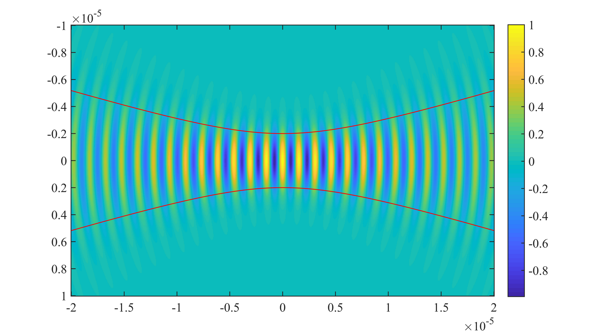 ※ 高斯光束在自由空间传播过程的电场分量实部的归一化分布
将上述代码的第 21 行改为:
1
| imagesc(zd,rd,abs(real(E)))
|
得到高斯光束在自由空间传播过程中的电场分量实部绝对值的归一化分布。该图更多地被用来展示高斯光束的电场分布形式。
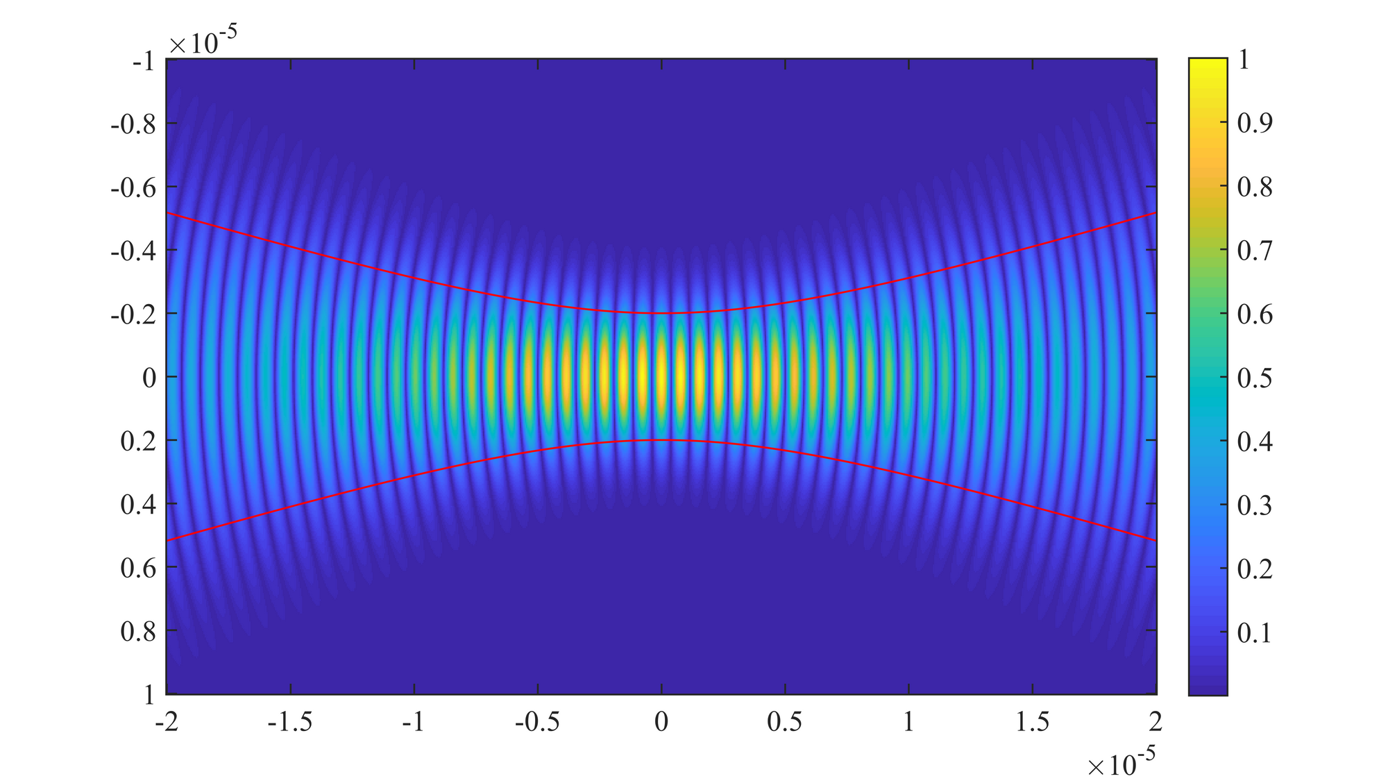 ※ 高斯光束在自由空间传播过程的电场分量实部绝对值的归一化分布
在上述代码的基础上,运行下面的程序,得到高斯光束咋自由空间传播的过程中电场分量的变化。
 1
 2
 3
 4
 5
 6
 7
 8
 9
10
11
12
13
14
15
16
17
18
19
20
21
| numFrames=25;
for k=1:numFrames
E=w0./w.*exp(-r.^2./w.^2).*exp(-(i*(k0*(r.^2./(2*R)+z)-phi-k*2*pi/25)));
E=E/(max(max(abs(E))));
imagesc(zd,rd,real(E))
hold on
plot(zd,w(1,:),'r',zd,-w(1,:),'r')
mov(k)=getframe;
end
VideoWriter('GaussianBeam.avi');
animated(1,1,1,numFrames)=0;
for k=1:numFrames
if k==1
[animated,cmap]=rgb2ind(mov(k).cdata,256,'nodither');
else
animated(:,:,1,k)=rgb2ind(mov(k).cdata,cmap,'nodither');
end
end
filename='GaussianBeam.gif';
imwrite(animated,cmap,filename,'DelayTime',0.1,'LoopCount',inf);
web(filename)
|
 ※ 高斯光束在自由空间传播过程中的电场分量变化
高斯光束通过薄透镜时,传播矩阵为:
$$
M=
\begin{bmatrix}
1&0\\
-1/f&1
\end{bmatrix}
$$
成像公式为:
$$
\frac{1}{s_i}=\frac{1}{f}-\frac{1}{s_0}\frac{1}{1+Z_{01}^2/s_0(s_0-f)}
$$
物像比例公式为:
$$
w_i=\frac{fw_0}{[(s_0-f)^2+Z_{01}^2]^{1/2}}
$$
作出高斯光束在通过薄透镜变换时,取不同的归一化参数 $Z_{01}/f$ $(0,0.2,0.4,0.5,1,5)$ 的情况下,归一化物距参数 $s_0/f$ 随归一化相距参数 $s_i/f$ 的变化曲线。
 1
 2
 3
 4
 5
 6
 7
 8
 9
10
11
12
13
14
15
16
17
18
19
20
| f=0.1;
Z0=[0 0.2 0.4 0.5 1 5]*f;
t=-2:0.01:4;
s1=f*t;
s2=zeros(length(t),length(Z0));
for i = 1:length(Z0)
s2(:,i) = f+(s1-f)*f^2./[(f-s1).^2+Z0(i).^2];
end
plot(s1/f,s2/f)
axis([-2 4 -2 4])
grid on
axis square
xlabel('s_0/f')
ylabel('s_i/f')
text(0.5,2.5,'z_{01}/f')
text(1.3,3.8,'0')
[val pos]=max(s2);
for i=2:length(Z0)
text(t(pos(i))-0.1,val(i)/f-0.1,num2str(Z0(i)/f));
end
|
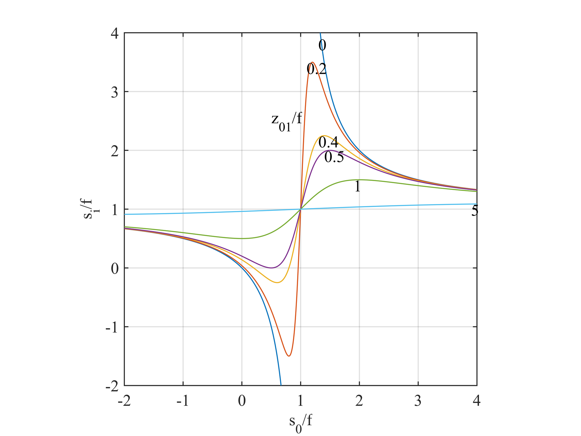 ※ 归一化像距和归一化物距的关系曲线
当 $(s_0-f)^2\gg Z_{01}^2$,$Z_{01}\rightarrow 0$时,成像公式过渡为几何光学中薄透镜的成像公式:
$$
\frac{1}{s_i}+\frac{1}{s_0}=\frac{1}{f}
$$
作出物像比例 $w_i/w_0$ 和归一化物距 $s_0/f$ 的关系曲线。
 1
 2
 3
 4
 5
 6
 7
 8
 9
10
11
12
13
14
15
16
17
18
19
20
21
| clear
f=0.1;
Z01=[0 0.2 0.4 0.5 1 2 5]*f;
t=-2:0.01:4;
s0=f*t;
w1w0=zeros(length(t),length(Z01));
for i=1:length(Z01)
w1w0(:,i)=f./sqrt((s0-f).^2+Z01(i)^2);
end
plot(s0/f,w1w0)
axis([-2 4 0 6])
grid on
axis square
xlabel('s_0/f')
ylabel('w_1/w_0')
text(0.2,3.5,'Z_{01}/f')
text(1,5.5,'0')
[val pos]=max(w1w0);
for i=2:length(Z01)
text(t(pos(i)),val(i),num2str(Z01(i)/f));
end
|
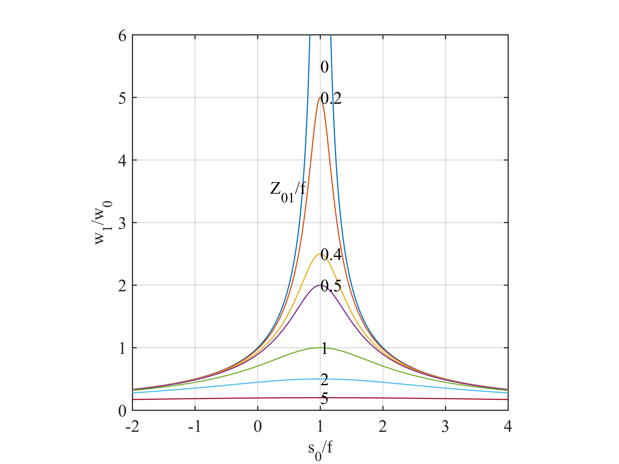 ※ 物像比例和归一化物距的关系曲线
当 $(s_0-f)^2\gg Z_{01}^2$,$Z_{01}\rightarrow 0$时,物像比例与几何光学相同,有:
$$
w_i=\frac{fw_0}{s_0-f}=\frac{sw_0}{s_0}
$$
像方瑞利长度 $Z_{02}$ 为:
$$
Z_{02}=\frac{\pi w_i^2}{\lambda}=\frac{f^2Z_{01}}{Z_{01}^2+(s_0-f)^2}
$$